7 Logistic Regression
7.1 Introduction
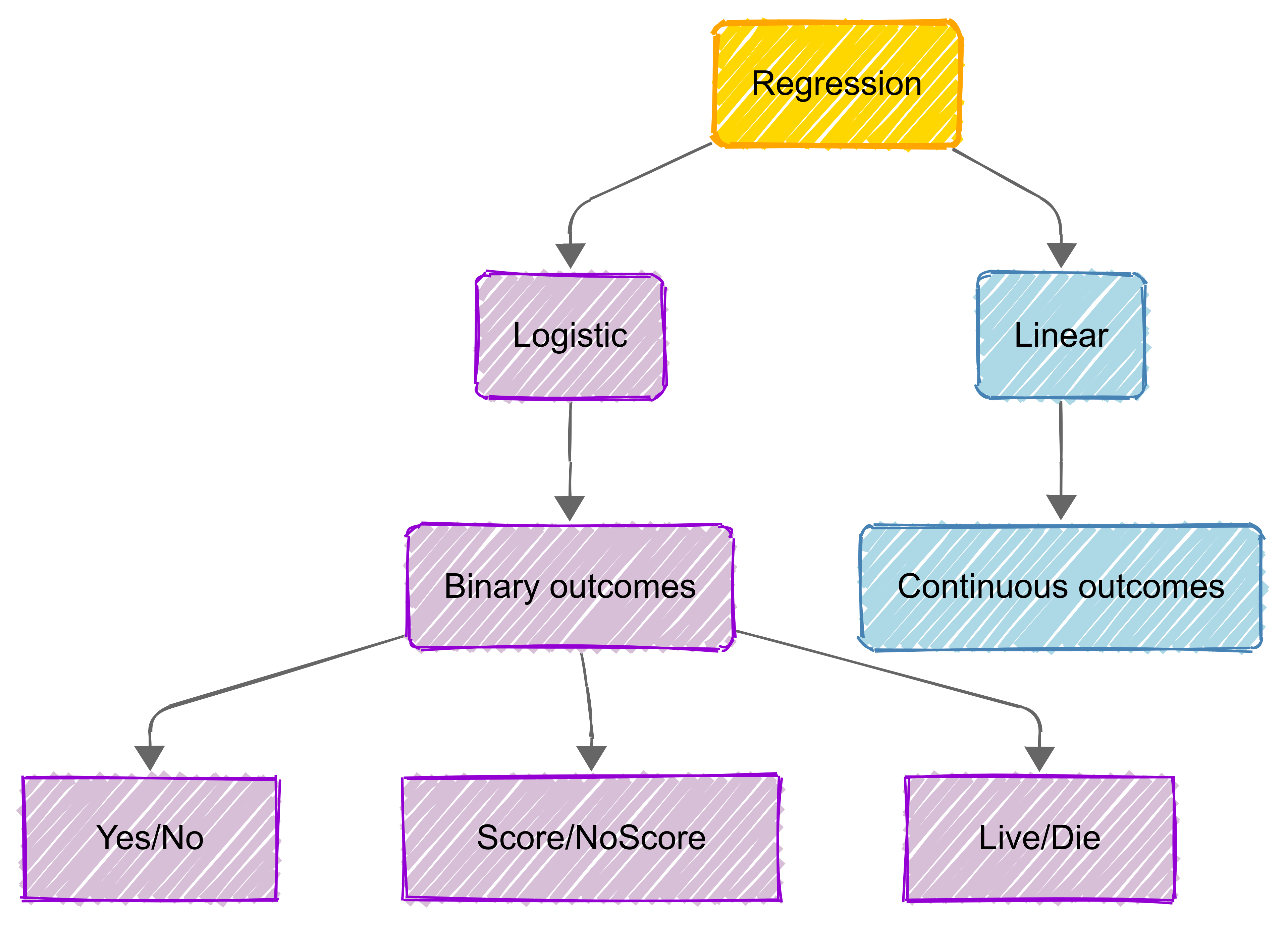
Logistic regression is a statistical method used when we want to model the probability of a binary (e.g., yes/no) outcome based on one or more predictor variables.
Unlike linear regression (such as Multiple Linear Regression) , which predicts continuous values, logistic regression specifically handles cases where the dependent variable is categorical and binary in nature.
This technique gets its name from the logistic function (also called the sigmoid function) that transforms any real-valued number into a value between 0 and 1, making it perfect for probability prediction.
.png)
The logistic model basically estimates the probability that an instance belongs to a particular category, either 0 or 1.
The power of logistic regression lies in its ability to handle multiple predictor variables, both continuous and categorical, while providing easily interpretable results in terms of odds ratios.
7.2 Key Concepts
Introduction
Logistic regression (LR) is a statistical method for binary classification.
There are four key concepts that are central to understanding LR:
Odds and Log Odds: These concepts form the basis of logistic regression, helping us understand how to transform probabilities into a more manageable form.
Probability Estimation: This is the process of calculating the likelihood of an outcome occurring, which is central to making predictions in logistic regression.
Sigmoid Function: The mathematical function that transforms linear predictions into probability values between 0 and 1, making it essential for binary classification tasks.
Binary vs. Multinomial Logistic Regression: Understanding the differences between these two types of logistic regression and when to apply each one.
Odds and log odds
In logistic regression, the odds represent the likelihood of an event occurring compared to it not occurring.
If \(p\) is the probability of success (e.g., a positive outcome), the odds are calculated as:
\[ Odds = \frac{p}{1 - p} \]
For example, if the probability of success is 0.8, the odds are \(\frac{0.8}{0.2} = 4\), meaning success is four times more likely than failure.
Log Odds (Logit Function)
Since odds are always positive and can grow exponentially, log odds (also called the logit function) transform them into a continuous scale that can take any real value:
\[ Log Odds = \log \left(\frac{p}{1 - p} \right) \]
Logistic regression models the relationship between predictor variables and the log ods of an outcome, making the response variable linear and suitable for regression analysis. The model equation is:
\[ \log \left(\frac{p}{1 - p} \right) = \beta_0 + \beta_1 x_1 + \beta_2 x_2 + \dots \]
Interpretation in Logistic Regression
Each coefficient (\(β\)) in the logistic regression model represents the change in log odds for a one-unit increase in the predictor variable. When exponentiated (\(e^β\)), the coefficient gives the odds ratio, indicating how much the odds of the event change for each unit increase in the predictor.
If an odds ratio is greater than 1, the predictor increases the likelihood of the outcome; if less than 1, it decreases it.
Example
Consider a logistic regression model predicting whether a student will pass an exam based on study hours. Suppose we get the following equation from our regression model:
\[ \log \left(\frac{p}{1-p}\right) = -2.5 + 0.8x \]
where \(x\) is the number of study hours.
We can interpret this as follows:
- The coefficient \(β_1 = 0.8\) means that for each additional hour of studying, the log odds of passing increase by 0.8;
- To find the odds ratio, we calculate \(e^{0.8} \approx 2.23\).
This means that for each additional hour of studying, the odds of passing the exam increase by a factor of 2.23, or about 123%.
For example, if a student studies for 3 hours, their log odds of passing would be:
\[ -2.5 + 0.8(3) = -0.1 \]
To convert this to probability, we use the inverse logit function:
\[ p = \frac{1}{1 + e^{0.1}} \approx 0.475 \]
Therefore, a student who studies for 3 hours has approximately a 47.5% chance of passing the exam.
Probability estimation
In logistic regression, the goal is to estimate the probability of an event occurring based on predictor variables.
Since probabilities range between 0 and 1, logistic regression models the probability using the sigmoid function, which ensures the output stays within this range. The probability of success (\(p\)) given predictor variables is:
\[ p = \frac{1}{1 + e^{-(\beta_0 + \beta_1 x_1 + \beta_2 x_2 + \dots)}} \]
This function transforms a linear combination of predictors into a probability, making logistic regression ideal for binary classification problems (e.g., predicting whether an email is spam or not).
Probability and Odds
Instead of predicting probability directly, logistic regression first estimates the log odds and then converts them into probability using the formula above.
The relationship between probability (\(p\)) and odds is:
\[ Odds = \frac{p}{1 - p} \]
Solving for \(p\):
\[ p = \frac{e^{(\beta_0 + \beta_1 x_1 + \dots)}}{1 + e^{(\beta_0 + \beta_1 x_1 + \dots)}} \]
This equation shows that as predictor values change, so does the probability of the outcome occurring.
Interpretation in Logistic Regression
The estimated probability helps in decision-making.
- If \(p\) is greater than a threshold (commonly 0.5), we classify the outcome as 1 (success); otherwise, it’s 0 (failure).
- The logistic model coefficients (\(β\)) influence how much each predictor contributes to increasing or decreasing the probability.
Sigmoid function
The sigmoid function is fundamental to logistic regression for several key reasons:
- It transforms linear predictions into probability values between 0 and 1, making it perfect for binary classification problems;
- The smooth, continuous nature of the function allows for effective gradient-based optimisation during model training; and
- Its derivative has a simple form, which makes it computationally efficient for calculating gradients in the learning process.
In logistic regression, the sigmoid function acts as the activation function that converts the linear combination of inputs (\(wx + b\)) into a probability estimate:
\[ P(y=1|x) = \frac{1}{1 + e^{-(wx + b)}} \]
This probability output can then be used to make binary predictions by applying a threshold (typically 0.5).
What is the Sigmoid Function?
The sigmoid function, also known as the logistic function, is an S-shaped curve that maps any real-valued number into a value between 0 and 1. It is defined by the formula:
\[ σ(x) = \frac{1}{1 + e^{-x}} \]
Applications
The sigmoid function is widely used in:
- Machine Learning, particularly in logistic regression and neural networks;
- Binary classification, for converting continuous values to binary outcomes; and
- Probability estimation, when modelling probability distributions. As we’ve covered, logistic regression is used for classification when the outcome is categorical.
Binary logistic regression applies when there are two categories (e.g., pass/fail, yes/no, 0/1), while multinomial logistic regression handles three or more categories (e.g., car, bus, train).
Binary Logistic Regression
In binary logistic regression, the model estimates the log odds of belonging to one category over the other using the formula:
\[ log \left(\frac{p}{1 - p}\right) = \beta_0 + \beta_1 x_1 + \dots \]
The output is a probability, which is converted into a class prediction using a threshold (usually 0.5). If p>0.5, the prediction is 1, otherwise 0. This is useful in cases like fraud detection or medical diagnosis.
Multinomial Logistic Regression
Multinomial logistic regression extends this to three or more categories, comparing each to a reference category. It estimates separate log odds equations, making it useful for customer segmentation, sentiment analysis, or species classification.
Unlike ordinal logistic regression, it does not assume any ranking between categories.
7.3 Model Fitting
.png)
In logistic regression, ‘model fitting’ is the process of determining the best values for the model’s coefficients to accurately predict the probability of a binary outcome.
For example, in predicting whether a basketball team will win a game (binary outcome), we need to find the best coefficient values for factors like average points scored, rebounds, and shooting percentage. If a team scores an average of 110 points with a 48% shooting percentage, these values would be used with their respective coefficients to calculate the probability of winning.
Basically, our goal is to align the model’s predicted probabilities with the observed data as closely as possible.
This is typically achieved using Maximum Likelihood Estimation (MLE), which finds the parameters that maximise the likelihood of observing the given data. When MLE cannot be solved analytically, numerical optimisation methods like Gradient Descent or Iterative Reweighted Least Squares (IRLS) are used.
A well-fitted model balances accuracy and generalisability, avoiding overfitting to the training data. Techniques like L1 (Lasso) and L2 (Ridge) regularisation further improve fitting by simplifying the model and addressing overfitting or multicollinearity. The gives us an interpretable model that reliably estimates the probability of an outcome based on predictor variables.
Maximum Likelihood Estimation
In logistic regression, MLE determines the probability of an event occurring based on the relationship between predictor variables and a binary outcome.
This involves maximising a likelihood function, which measures how well the model fits the data. Once the best-fitting parameters are identified, the model can predict probabilities of outcomes with greater accuracy.
.png)
Gradient Descent
.png)
“Gradient Descent” is an optimisation algorithm used to estimate the coefficients in logistic regression, particularly when Maximum Likelihood Estimation cannot be solved analytically.
The method works iteratively: it starts with initial guesses for the parameters and gradually updates them by moving in the direction that reduces the model’s error. The “gradient” indicates the slope or rate of change of the loss function, guiding how the parameters are adjusted.
Step size, or learning rate, is crucial to ensure the method converges efficiently to the optimal solution without overshooting or stalling.
Gradient Descent is especially useful when we’re dealing with large datasets or complex models.
Iterative Reweighted Least Squares
Iterative Reweighted Least Squares (IRLS) is a numerical method for solving logistic regression by approximating the maximum likelihood estimates of the parameters.
Unlike ordinary least squares used in linear regression, logistic regression involves a nonlinear relationship, so IRLS works iteratively. At each step, it “reweights” the data based on the current predictions and solves a weighted least squares problem.
This process continues until the parameters converge to a stable solution. IRLS is particularly effective for fitting logistic regression models as it combines efficiency with accuracy.
.png)
Regularisation (L1, L2)
Regularisation techniques help improve the performance of logistic regression models by preventing overfitting, where the model learns the noise in the data rather than the true relationship.
L1 regularisation, or Lasso, adds a penalty proportional to the absolute value of the coefficients, encouraging some coefficients to become zero, which simplifies the model.
In simpler terms, L1 regularisation adds or removes features from the model by making some coefficients exactly zero
L2 regularisation, or Ridge, adds a penalty proportional to the square of the coefficients, shrinking them towards zero but not eliminating them.
Both techniques strike a balance between model fit and complexity, improving generalisability of our models to new data.
7.4 Model Evaluation
Confusion matrix
A confusion matrix is a tool used to evaluate the performance of a classification model by comparing predicted and actual class labels. It summarises the model’s predictions into four key categories:
True Positives (TP) – Correctly predicted positive cases;
True Negatives (TN) – Correctly predicted negative cases;
False Positives (FP) – Incorrectly predicted as positive (Type I error); and
False Negatives (FN) – Incorrectly predicted as negative (Type II error).
From this matrix, we can derive important evaluation metrics like accuracy, precision, recall, and F1-score, which provide deeper insight into model performance beyond overall accuracy.
.png)
Why use a confusion matrix?
Accuracy alone can be misleading, especially in imbalanced datasets, where one class is much more frequent than the other. The confusion matrix allows for a more nuanced assessment, helping to determine whether the model is biased towards a particular class.
Precision and recall are particularly useful when false positives or false negatives have different real-world consequences, such as in medical diagnosis or fraud detection.
ROC Curve and AUC
The Receiver Operating Characteristic (ROC) curve is a graphical tool for evaluating the performance of a binary classification model.
It plots the True Positive Rate (Sensitivity) against the False Positive Rate (1 - Specificity) at different classification thresholds. A well-performing model has a curve that bends towards the top-left corner, indicating high sensitivity with low false positives.
.png)
The Area Under the Curve (AUC) quantifies overall model performance. AUC values range from 0 to 1:
AUC = 1: Perfect classifier.
AUC > 0.8: Strong model.
AUC = 0.5: No predictive power (random guessing).
A higher AUC means better discrimination between classes.
.png)
Precision and Recall
Precision and recall are key metrics for evaluating the performance of a logistic regression model, especially when dealing with imbalanced datasets where accuracy alone can be misleading.
These metrics are derived from the confusion matrix and help assess how well the model distinguishes between the two classes.
Precision: Measuring Predictive Accuracy
Precision (also called Positive Predictive Value) measures the proportion of correctly predicted positive cases out of all predicted positives:
\[ Precision = \frac{TP}{TP + FP} \]
A high precision means that when the model predicts a positive outcome, it is usually correct. This is critical in applications where false positives are costly, such as fraud detection or spam filtering (where you don’t want to wrongly classify a legitimate email as spam).
Recall: capturing all positive cases
Recall (also known as Sensitivity or True Positive Rate) measures the proportion of actual positives that were correctly predicted:
\[ Recall = \frac{TP}{TP + FN} \]
A high recall means the model correctly identifies most of the actual positive cases, which is important in scenarios like medical diagnosis, where failing to detect a disease (false negative) can have serious consequences.
Balancing precision and recall
There is often a trade-off between precision and recall, as increasing one may decrease the other. The F1-score, defined as the harmonic mean of precision and recall, helps balance both:
\[ F1 = 2 \times \frac{\text{Precision} \times \text{Recall}}{\text{Precision} + \text{Recall}} \]
A well-calibrated logistic regression model finds the right balance based on the problem at hand. For example:
In spam detection, precision may be prioritised to avoid flagging important emails incorrectly.
In healthcare, recall may be more important to ensure no positive cases are missed.
By tuning the classification threshold, we can optimize for either precision or recall, depending on the specific requirements of the task.
7.5 Feature Engineering
Introduction
“Feature engineering” is the process of creating, transforming, and selecting input variables (features) to improve a model’s performance.
It involves transforming raw data into features that better represent the underlying problem, making it easier for the logistic regression model to learn patterns and make accurate predictions.
Some of the goals of feature engineering in logistic regression are:
Making features more suitable for the linear nature of logistic regression;
Capturing important relationships and patterns in the data;
Improving model performance and predictive accuracy; and
Reducing noise and irrelevant information in the data.
Common techniques in logistic regression include scaling numerical features, encoding categorical variables, creating interaction terms, and handling missing values.
Feature Scaling
As we discussed earlier in the module, feature scaling is the process of standardising or normalising numerical input variables to ensure that they are on a similar scale.
While logistic regression does not require feature scaling for model accuracy (since it’s not distance-based like k-NN or Support Vector Machines), scaling can still improve optimisation and model performance in certain scenarios.
Why is Feature Scaling Important?
Improves Convergence Speed – logistic regression is trained using gradient descent, which can be slow when features have vastly different scales. Scaling helps gradient descent converge faster and more smoothly.
Prevents Numerical Instability – large feature values can cause computational issues when calculating the log odds in logistic regression. Scaling reduces this risk.
Enhances Interpretability with Regularisation – when using L1 (Lasso) or L2 (Ridge) regularisation, scaling ensures that all features contribute equally to the penalty term, preventing features with larger magnitudes from dominating the model.
Common feature scaling methods
Min-Max Scaling: Rescales values to a range of [0,1]:
\[ x' = \frac{x - \min(x)}{\max(x) - \min(x)} \]
Standardisation (Z-score normalisation): Transforms data to have a mean of 0 and standard deviation of 1:
\[ x′=x−μσx' = \frac{x - \mu}{\sigma} \]
When to scale features in Logistic Regression
If using gradient-based optimisation (e.g., SGD).
When applying regularisation (L1 or L2 penalty).
When feature magnitudes vary significantly.
While not always necessary, feature scaling can improve efficiency and stability, making it a useful pre-processing step in logistic regression.
Interaction Terms
Interaction terms in logistic regression are features created by multiplying two or more existing features together.
They capture how the relationship between one predictor variable and the target depends on the value of another predictor variable.
They help model non-linear relationships that can’t be captured by individual features alone, and can significantly improve model performance when features have interdependent effects on the outcome
Common examples of interactions include [age and income], [price and quantity], or [temperature and humidity].
Interaction terms must used carefully to avoid overfitting, and to maintain model interpretability
The decision to include interaction terms should be guided by your domain knowledge and statistical testing, as they increase model complexity and can make interpretation more challenging.
Polynomial Features
Polynomial features transform the original input variables into higher-degree terms, allowing logistic regression to capture nonlinear relationships between features and the target variable.
While standard logistic regression models linear decision boundaries, adding polynomial terms can introduce curvature, making the model more flexible for complex datasets.
How polynomial features work
Given an input feature \(x\), polynomial transformation creates additional features:
For degree 2:
\[ (x) \quad \rightarrow \quad (x, x^2) \]
For degree 3:
\[ (x) \quad \rightarrow \quad (x, x^2, x^3) \]
For multiple features $(x_1, x_2),$ it also includes interaction terms:
\[ (x_1, x_2) \quad \rightarrow \quad (x_1, x_2, x_1^2, x_2^2, x_1 x_2) \]
Why use polynomial features in Logistic Regression?
Handles Nonlinearity – If the relationship between predictors and the outcome is not purely linear, polynomial features allow logistic regression to fit more complex decision boundaries.
Enhances Model Flexibility – Captures interactions and curved relationships without needing a non-linear model like neural networks.
Works with Regularization – Polynomial terms can be penalised with L1/L2 regularisation to prevent overfitting.
Limitations
Computational Complexity – Higher-degree polynomials create many new features, increasing model complexity and computation time.
Overfitting Risk – Too many polynomial terms can cause the model to fit noise in the training data instead of generalising well.
Feature Scaling Needed – Polynomial features often lead to large feature magnitudes, so scaling is recommended to improve optimisation stability.
When to use polynomial features
When data exhibits curved decision boundaries rather than a simple linear separation.
When nonlinear relationships between features and the target are suspected.
When simpler models (like logistic regression) are preferred over more complex alternatives like neural networks or decision trees.
Polynomial features expand logistic regression’s capability beyond linear classification, but careful regularisation and feature selection are needed to avoid overfitting.
Handling categorical variables
Logistic regression requires numerical input features, so categorical variables must be transformed into a suitable format before being used in the model.
This process, known as feature engineering for categorical variables, ensures that the model can correctly interpret non-numeric data while preserving meaningful relationships.
Common Methods for Encoding Categorical Variables
One-Hot Encoding (Dummy Variables)
One-hot encoding creates binary (0/1) variables for each category. For a categorical feature like Colour (Red, Blue, Green), it transforms into:
| Colour | Red | Blue | Green | |||||
| Red | 1 | 0 | 0 | |||||
| Blue | 0 | 1 | 0 | |||||
| Green | 0 | 0 | 1 |
Pros: Works well for nominal (unordered) categories.
Cons: Increases dimensionality when there are many unique categories.
To avoid redundancy, one column is usually dropped (e.g., drop “Green”) to prevent perfect multicollinearity.
Ordinal Encoding (Integer Encoding)
For ordinal variables (where categories have a meaningful order), values are mapped to integers. Example for Size (Small, Medium, Large):
| Size | Encoded Value | |||
| Small | 1 | |||
| Medium | 2 | |||
| Large | 3 |
Pros: Retains the order of categories.
Cons: Assumes that the numeric distances between categories are meaningful, which may not always be the case.
Frequency Encoding
Replaces each category with its frequency in the dataset.
Example for Product Category:
|—–|————-|—–|—————|—–| | | Product | | Frequency | | | | A | | 0.4 | | | | B | | 0.3 | | | | C | | 0.3 | |
Pros: Captures the importance of each category.
Cons: May introduce bias if category frequencies are too influential.
Choosing the right encoding method
Nominal variables → One-Hot Encoding
Ordinal variables → Ordinal Encoding
High-cardinality variables → Frequency Encoding or Target Encoding (using mean outcomes per category)